QGIS for Interpolation of Spatial Data

Introduction to Interpolation Process for Spatial Analysis

Continuous spatial data is very important in many applications for spatial analysis. So for such analysis, acquiring continuous spatial data is very difficult, costly and usually takes very long time for study area. 

In case, if one needs to collect/create continuous data then field sampling and observations is very common practice, such as water sampling for quality analysis. But during this field sampling process, it is nearly impossible to collect data from each and every spot of field, usually samples collected at certain distance. 

So this distance gap/interval between two samples/more samples is not possible to cover as well as very tedious and time consuming. In this case, some representative samples such as water samples from all well locations or pollution parameters from air monitoring stations will be collected and interpolation method is deployed to create continuous layer. 

Accuracy of interpolated spatial data depends upon the quantity and spatial distribution of collected samples.

There are several methods are used for interpolation and most commonly used interpolation technique is ‘Inverse Distance Weighted (IDW)’

IDW using QGIS

‘Inverse Distance Weighted (IDW)’ is a method that used to estimate the interpolated values on location, which are not sampled during survey. In this process, value at intermediate locations, which do not have known values calculated by an inverse function of distance from the known value of samples points.

In this article, interpolation method using QGIS is explained. Below is the process of Interpolation in GIS environment.

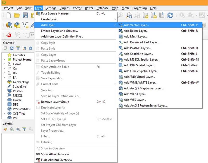
1. Open ‘point data’ shapefile in QGIS, for this click on Menu then Layer followed by Add Vector Layer as shown below

The Data Source Manager-Vector window will pop up.

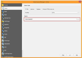
Here One have to Browse (for the point data folder) and select the point shape file. Then click on Add button and close the window.

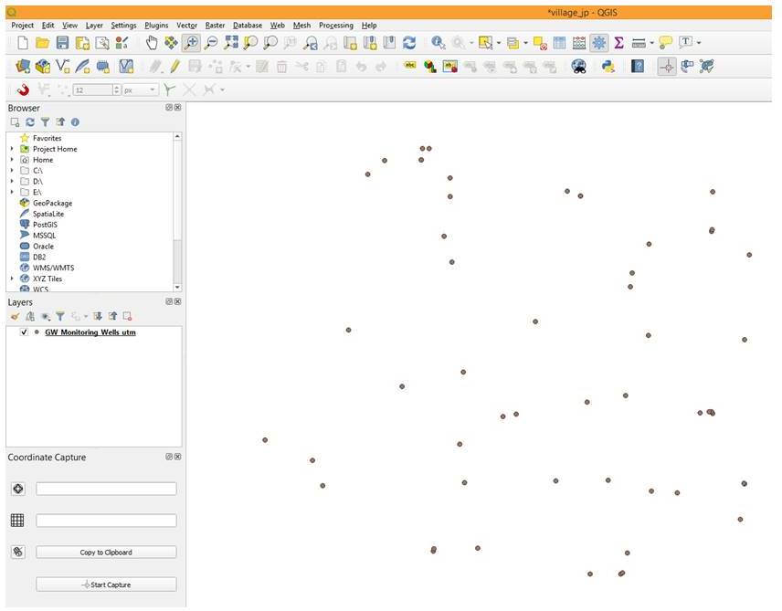
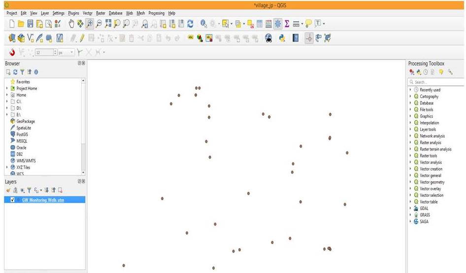
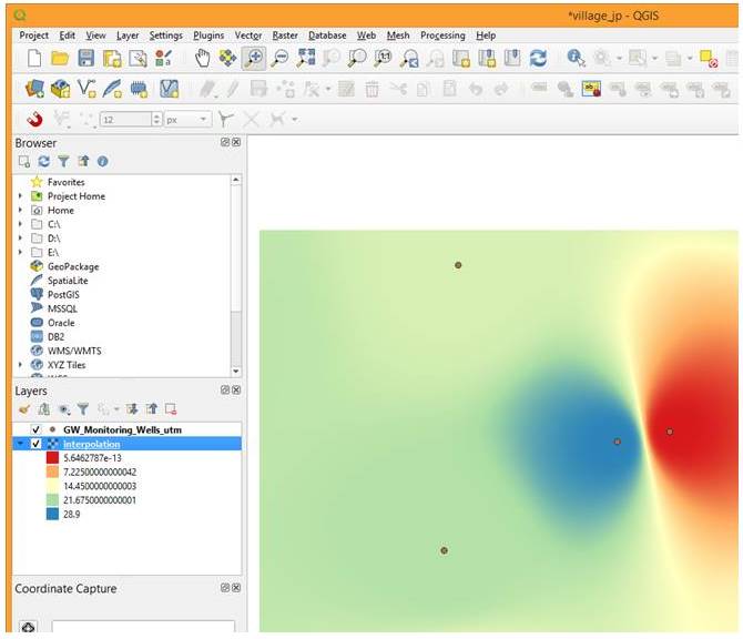
For example here we have opened the Ground water monitoring wells point shapefile, and points are displayed on the screen as shown below

2. Now one have to open the attribute table of your point layer by Right click on point shapefile under Layer section and select ‘Open Attribute Table’. It will open the attribute table of shape file.

For example: Right click on ‘GW_Monitoring_Wells_utm.shp’ under Layer section and select ‘Open Attribute Table’. 

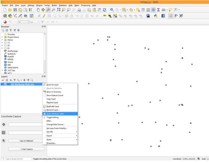
It will open the attribute table of point shapefile, which contains different parameters. Here you can see that for which one parameter one want to create spatial distribution map using IDW Interpolation technique. Now you can Close the attribute table.

3. Click on Menu then Processing followed by Tool box as shown below

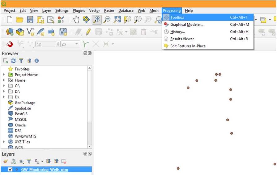
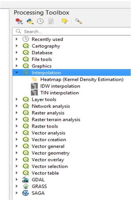
Processing Tool box will open on the right side of the screen as shown below

Now click on Interpolation it will show three techniques viz Heatmap, IDW Interpolation and TIN Interpolation

Now click on IDW Interpolation, following window will pop up. Here select point shapefile in Vector layer

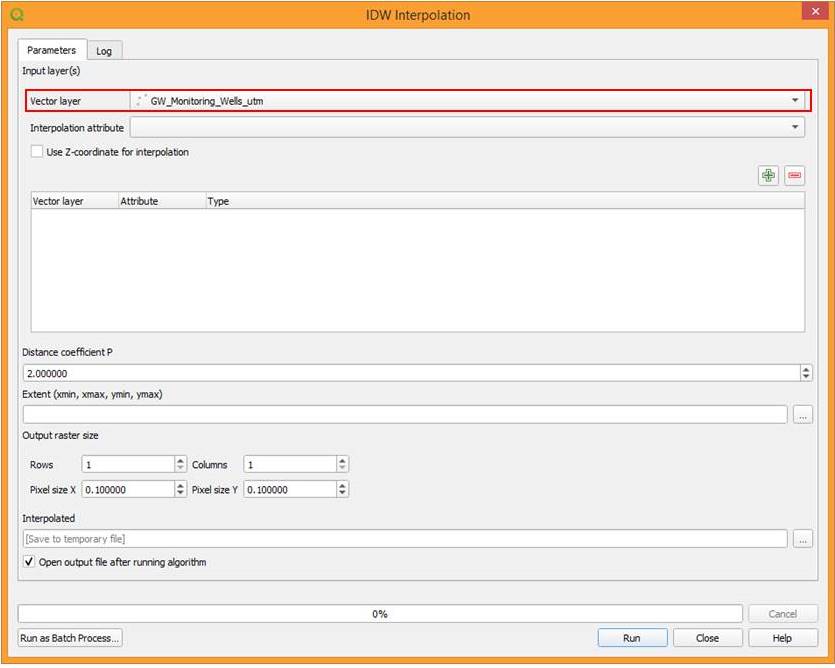
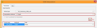
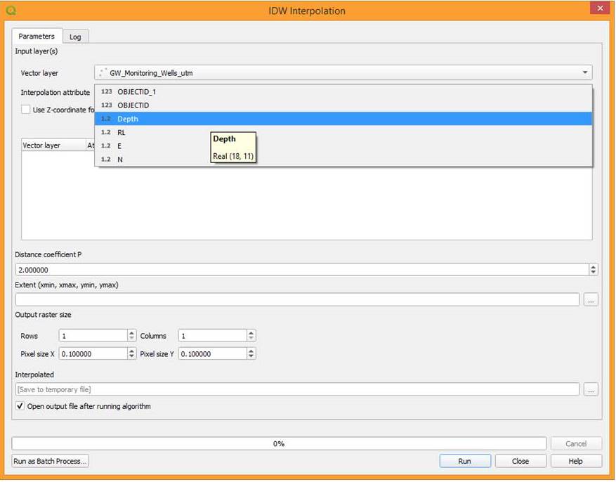
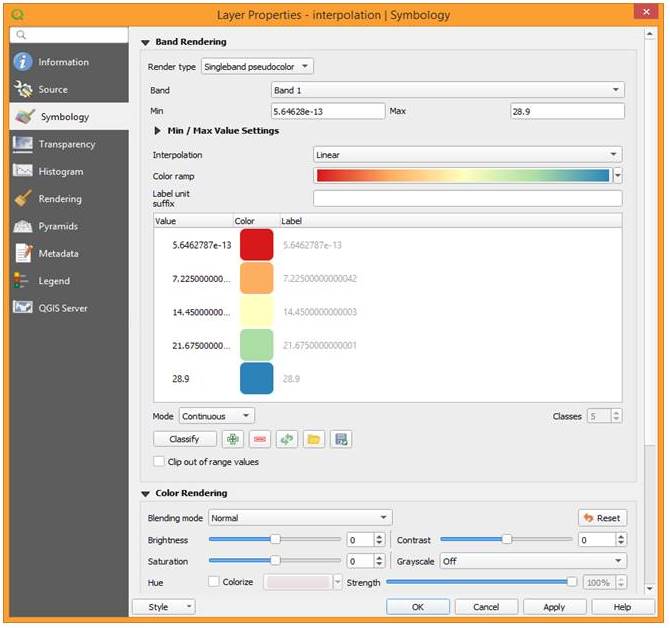
In Interpolation attribute specify the parameter need to be interpolated. Here we have selected Depth. After selecting the attribute click on ‘Add’ button just below it. Now ‘Depth’ is added for interpolation.

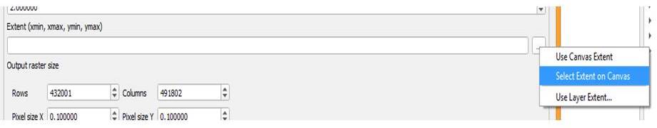
Now define the extent and click on select extent on canvas as shown below. For this you have to draw box on screen and it will automatically take the extent values. Another option is that you can define extent by clicking on use layer extent.

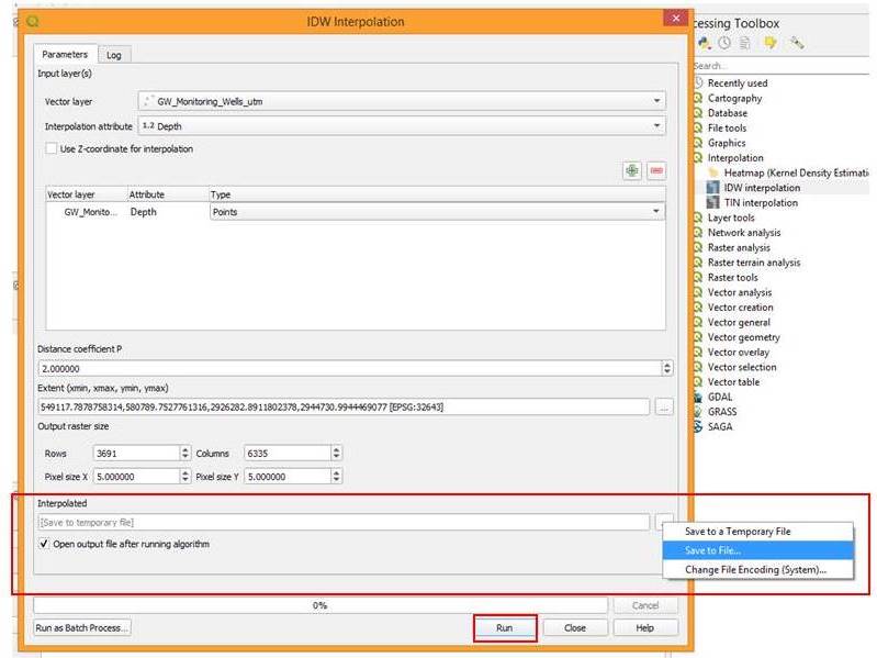
 Now specify the pixel size for X and Y.

Finally specify the output file name in the folder created by you to get the interpolated output. Don’t forget to check the check box ‘open output file after running algorithm’. Click ‘Run’.

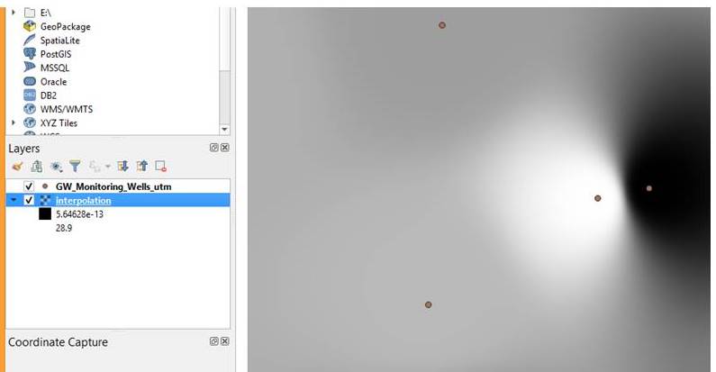
After processing, you will notice interpolated output file added to the map canvas. The output will be displayed in black and white/grayscale but you can try different

color ramp to make it more legible. 

For this you have to go to the Layer properties by right click on output file under Layer section and select Properties. Do the changes in Symbology window and get the colored map with appropriate legend.

This interpolation method can be used in many ways for spatial analysis some examples are shared below:

Spatial Pattern of Drinking Water

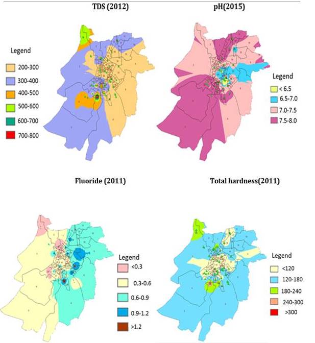
• The spatial distribution maps of various physico-chemical parameters 
• such as pH, Total dissolved solids, Total hardness, and Fluoride were created at ward level as shown below 

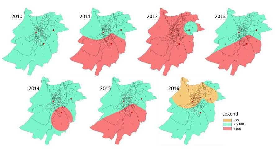
Spatial and temporal changes in Air Quality

• Spatial distribution of air quality in Kota city
• The AQI values were interpolated and calculated
• Spatial patterns of air pollution created through interpolation process
• The AQI values so derived was divided into five categories i.e.
• 0 -25 = Clean air, 
• 26-50 = Light air pollution, 
• 51-75 = Moderate air pollution, 
• 76-100 = Heavy air pollution 
• and the value above 100 signifies severe air pollution.

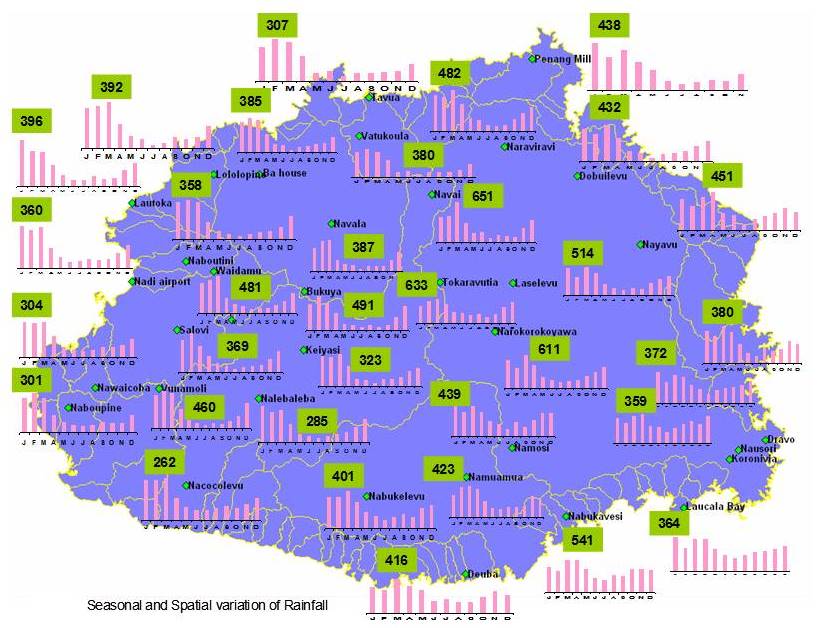
Rainfall Analysis

• Total 35 stations were selected for the rainfall analysis.
• The daily rainfall data from 1976 to 2008 was analyzed
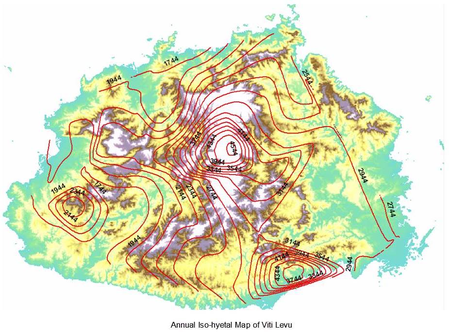
• Average monthly and annual rainfall was computed and annual iso-hyetal map was determined
• seasonal and spatial variation of rainfall estimated through interpolation method